Global maps & projections

Gridded layers loaded with load_layer (fmt="xarray") plot in a single line. The examples below use the plotting extra:

pip install "pyo-oracle[viz]"

A coarse global subset

The native grid is 0.05°, so for a global view we stride over it with latitude_step / longitude_step to keep the download small.

import pyo_oracle as pyo

ds_id = "thetao_baseline_2000_2019_depthsurf"
constraints = pyo.build_constraints(
    ds_id,
    latitude=(-89.975, 89.975),
    longitude=(-179.975, 179.975),
    latitude_step=20,   # ~1° grid
    longitude_step=20,
)
ds = pyo.load_layer(ds_id, constraints=constraints, variables=["thetao_mean"], fmt="xarray")

Quick map

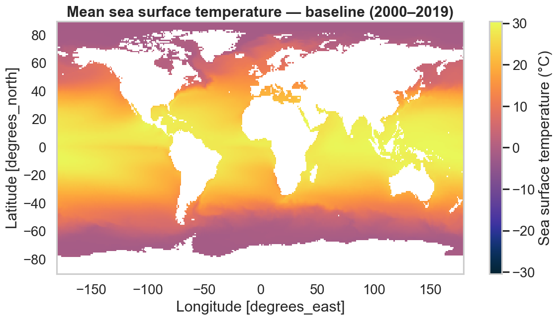
xarray's .plot() picks a sensible 2-D map automatically. Swap in a cmocean colormap for an oceanographic look.

import cmocean
import matplotlib.pyplot as plt

ds["thetao_mean"].isel(time=0).plot(
    figsize=(11, 5.5),
    cmap=cmocean.cm.thermal,
    cbar_kwargs={"label": "Sea surface temperature (°C)"},
)
plt.title("Mean sea surface temperature — baseline (2000–2019)")

Publication-quality projection

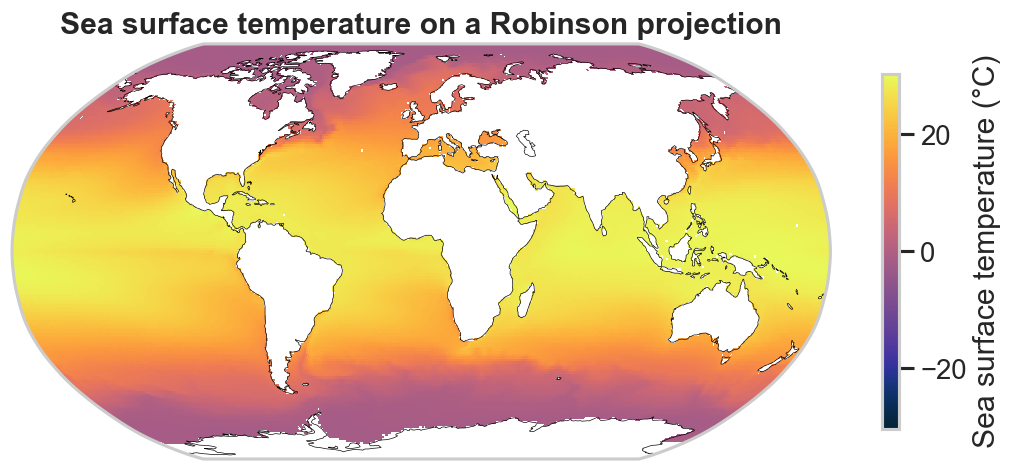
For coastlines and a proper map projection, hand the same DataArray to a cartopy axis. The key is transform=ccrs.PlateCarree() — it tells cartopy the data is on a regular lon/lat grid.

import cartopy.crs as ccrs

ax = plt.axes(projection=ccrs.Robinson())
ds["thetao_mean"].isel(time=0).plot(
    ax=ax,
    transform=ccrs.PlateCarree(),
    cmap=cmocean.cm.thermal,
    cbar_kwargs={"label": "Sea surface temperature (°C)", "shrink": 0.7},
)
ax.coastlines(linewidth=0.4)
ax.set_global()

Zoom into a region

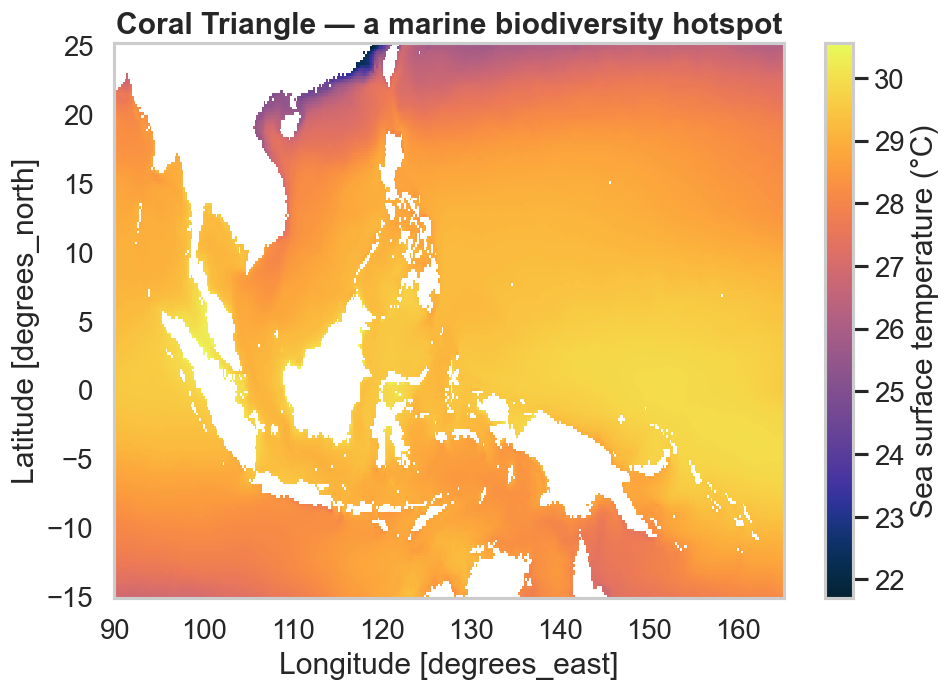
Pass tighter bounds with a finer step to study a single area — here the Coral Triangle, the planet's richest marine biodiversity hotspot.

constraints = pyo.build_constraints(
    ds_id,
    latitude=(-15, 25),
    longitude=(90, 165),
    latitude_step=4,    # ~0.2° grid
    longitude_step=4,
)
region = pyo.load_layer(ds_id, constraints=constraints, variables=["thetao_mean"], fmt="xarray")
region["thetao_mean"].isel(time=0).plot.pcolormesh(figsize=(9, 6), cmap=cmocean.cm.thermal)

Resolution vs. download size

Smaller *_step values mean finer maps but larger requests. Start coarse while exploring, then refine the step (or the bounding box) for the final figure.